Training JEPA World Models for Robots
A small robotics study of latent prediction, structured action proposals, event-scale dynamics, and hierarchy.
Recently, I decided to build a more forward-looking project and landed on world models, which are becoming the next horizon in ML research. Many AI pioneers, including Yann LeCun and Fei-Fei Li, are betting on them. This could enable a broad new class of physical automation.
Given my limited compute access, I decided to experiment with Yann LeCun’s paradigm, the Joint Embedding Predictive Architecture (JEPA). It works as follows:
- Learn useful representations, not pixels: Use self-supervised learning (SSL) to encode observations into abstract representations that capture meaningful structure while ignoring unpredictable details.
- Predict in latent space: Given the current context, predict the representation of a future or missing state rather than reconstructing every low-level detail.
- Plan with an internal world model: Use these predictions to evaluate possible actions, choose those likely to reach a desired outcome, and replan as new observations arrive.
Recent JEPA-based control studies have demonstrated latent planning on tasks such as pushing and maze navigation, but reliable planning through contact-rich, high-dimensional dynamics remains difficult.
To apply the paradigm at a larger scale, I trained action-conditioned JEPA world models and corresponding controllers to see how far they could go with contact, momentum, long horizons, and dexterous manipulation. The models use low-dimensional simulator state rather than pixels, and they are all under 10 million parameters.
These models were trained and tested on several tasks in Gymnasium Robotics. The experiments focus on whether compact latent models can support control across reaching, pushing, locomotion, and dexterous manipulation tasks.
The code and exact experiment ledger are available as open source in my GitHub repository, Mini-JEPA.
The model
A JEPA predicts in representation space instead of reconstructing the entire future observation. The general joint-embedding idea was introduced by Assran et al.
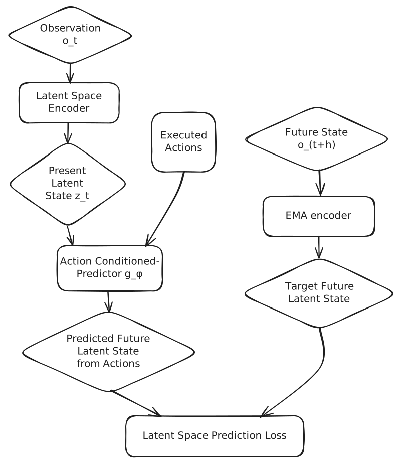
Let $o_t$ be the normalized observation and let $\mathbf a_{t:t+h-1}$ be an action sequence. The online encoder produces the current latent,
\[z_t = f_\theta(o_t),\]while an exponential moving average target encoder produces the regression target,
\[\bar z_{t+h} = f_{\bar\theta}(o_{t+h}), \qquad \bar\theta \leftarrow \mu\bar\theta + (1-\mu)\theta.\]The recurrent predictor rolls the latent forward under the action sequence:
\[\hat z_{t+i} = g_\phi\!\left(\hat z_{t+i-1},\, a_{t+i-1},\, i/h_{\max}\right), \qquad \hat z_t=z_t.\]The main predictive loss compares normalized latents at several horizons:
\[\mathcal L_{\mathrm{pred}} = \frac{1}{|\mathcal H|} \sum_{h\in\mathcal H} \left\| \frac{\hat z_{t+h}}{\|\hat z_{t+h}\|_2} - \frac{\bar z_{t+h}}{\|\bar z_{t+h}\|_2} \right\|_2^2 .\]Variance and off-diagonal covariance penalties keep the representation from collapsing, following the useful part of the VICReg recipe
This model is genuinely useful on smooth, locally controllable dynamics. On FetchReach, latent model-predictive control (MPC) can optimize primitive action sequences directly. This shows that, when dynamics are smooth and locally controllable, the predictor can evaluate candidate action sequences well enough for direct planning.
Where the data came from
Data collection is part of the method, not bookkeeping. There are two distinct roles for data in these experiments:
- world-model transitions provide tuples $(o_t,\mathbf a_{t:t+h-1},o_{t+h})$ for learning latent dynamics;
- behavior data provides the action chunks used to train inverse or flow proposal models and to identify useful phases or subgoals.
The exact source depends on the task:
| Task | World-model data | Proposal or hierarchy data |
|---|---|---|
| FetchReach | A mixture of scripted and random interaction with action noise | None for the pure latent-MPC controller |
| FetchPush / FetchPickAndPlace | Noisy scripted/random trajectories; the default recipe collects 400k transitions per task | Separate, more expert-heavy banks: 100k mostly scripted transitions for Push and 80k scripted transitions for Pick |
| FetchSlide | Scripted pre-alignment followed by a structured sweep over strike angle, amplitude, and duration | The same planned strikes, including misses, plus one round of planner-selected calibration data |
| PointMaze | Trajectories from a scripted maze controller | Route windows and local action chunks extracted from those trajectories |
| Adroit / Kitchen | Offline expert demonstrations from the D4RL reinforcement-learning benchmark, imported through Minari | Demonstration segments split by contact regime, possession, subtask completion, or handoff boundaries |
Keeping unsuccessful Slide strikes is especially important: endpoint prediction needs the response surface around a good strike, not only successful examples. For Kitchen, demonstrations are replayed and aligned with object-state changes to label subtask segments. The completion probe is learned from the aligned trajectories, while the handoff graph is constructed from demonstration-boundary distances.
JEPA targets and future indices are self-supervised. Phase labels and handoff costs are derived from trajectory boundaries and state changes. The action priors, however, are trained on the actions recorded in those trajectories.
Controller training does not use environment reward labels, critics, or value targets. It does, however, use expert demonstration actions, task geometry, and, for FetchSlide, goal-distance-based data balancing. The pipeline is therefore reward-label-free, not task-supervision-free. Random exploration did not discover grasping, dexterity, or Kitchen task sequences.
Overall, this is self-supervised representation learning plus trajectory-supervised action modeling.
Evaluation uses fresh rollouts with random seeds that were not used during training. The learned controllers do not receive scripted expert actions at test time; the scripted policies are data-collection tools, not hidden components of the reported controllers.
Separating Prediction and Control
Consider an example where a planner evaluates $N$ action chunks. Even a perfect world model can only choose among those $N$ candidates. If none contains a coherent grasp or push, prediction quality does not help.
This becomes severe with temporally precise contact. A useful grasp is a tiny region in a high-dimensional action-sequence space. Sampling each action from a wide Gaussian almost never enters that region, and local optimization receives little signal before contact occurs.
The successful controllers therefore separate two jobs:
- a proposal model samples action chunks that resemble feasible behavior;
- the JEPA predictor estimates what each proposed chunk will cause.
Recent work such as Subgoal-Conditioned Action Generation (SAGE) makes the same proposal-versus-evaluation distinction explicit for latent world-model planning
For relatively unimodal transitions, a deterministic inverse model predicts a chunk directly:
\[q_\omega(z_t,\bar z_{t+h},h,\gamma_t) \longrightarrow \hat{\mathbf a}_{t:t+H-1},\]where $\gamma_t$ contains a small amount of task geometry. This works well for FetchPickAndPlace once a future transition specifies the grasp-and-lift direction.
For multimodal transitions, I used conditional flow matching
the network learns the velocity
\[\mathcal L_{\mathrm{flow}} = \left\| v_\psi(\mathbf a_\tau,\tau\mid c) - (\mathbf a_1-\mathbf a_0) \right\|_2^2,\]conditioned on
\[c=[z_t,\bar z_{t+h},h,\gamma_t].\]Flow matching is useful when one condition admits several coherent action chunks. In FetchPush and the maze controllers, different pushes or route segments can remain feasible from the same state and goal; the flow retains those alternatives for JEPA to evaluate. For tightly specified contact phases in PickAndPlace, Relocate, and Kitchen, a future-conditioned inverse model is more appropriate because the demonstrated local transition is comparatively narrow.
At runtime, FetchPush samples complete action chunks from its flow prior, while FetchPickAndPlace generates local variants around the output of its deterministic inverse model. In both cases, the frozen JEPA rolls the candidate chunks forward and selects
\[\mathbf a^\star = \underset{\mathbf a^{(i)}\in\mathcal C(c)}{\arg\min} \left[ \lambda_z d\!\left(\hat z_{t+H}^{(i)},z_{\mathrm{target}}\right) + \lambda_x d_x\!\left(\hat o_{t+H}^{(i)},o_{\mathrm{target}}\right) + \lambda_\Delta R(\mathbf a^{(i)}) \right].\]Here, $\mathcal C(c)$ is the candidate set produced by the relevant proposal model under condition $c$.
The latent term checks representation-space agreement, the decoded-state term checks task geometry, and $R$ discourages unnecessarily large or discontinuous actions. Only the first few actions are executed before replanning.
This division of labor solved two contact tasks:
- FetchPush: a flow prior proposes coherent eight-step pushes; JEPA ranks them. The checked 30-episode run reached 1.00 success with about 8 mm mean final distance.
- FetchPickAndPlace: a future-conditioned inverse prior proposes grasp-and-lift chunks; JEPA ranks local variants. The checked 30-episode run reached 1.00 success with about 11 mm mean final distance.
The important point is not that flow matching is always better than an inverse multilayer perceptron (MLP). The important point is that the proposal distribution is part of the controller. Deterministic inverse models are useful when the inverse is nearly single-valued; flows are useful when several action sequences can realize the same future.
Ballistic world models
FetchSlide produced the clearest change in architecture.
The goal lies outside the robot’s reach. The gripper must hit a puck, withdraw, and let the puck coast under friction. Once the impact is over, there is little corrective authority. A controller that replans every few simulator frames is using the wrong unit of time.
The correct high-level transition is not
\[o_t \rightarrow o_{t+1}\rightarrow\cdots\rightarrow o_{t+24}.\]It is
\[\text{aligned pre-impact state} \xrightarrow{\text{planned strike}} \text{post-coast resting state}.\]The model has two parts. First, it converts the physical situation into goal-aligned coordinates; second, it combines those canonical features with the JEPA latent in an ensemble MLP that predicts where the puck will stop.
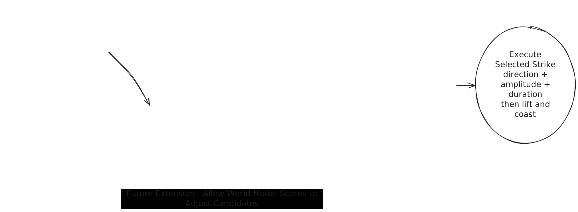
For each hit, the strike command is
\[m=[d_x,d_y,\alpha,\tau/\tau_{\max}],\]containing direction, strength, and duration. The coordinate frame points forward from the puck to the goal,
\[e_\parallel = \frac{p_{\mathrm{goal}}-p_{\mathrm{puck}}} {\|p_{\mathrm{goal}}-p_{\mathrm{puck}}\|_2}, \qquad e_\perp=[-e_{\parallel,y},e_{\parallel,x}].\]Every planar physical vector, including the gripper’s offset and velocity, the puck velocity, and the strike direction, is projected onto $(e_\parallel,e_\perp)$. Its first coordinate now means toward the goal and its second means sideways. A strike toward the goal therefore has nearly the same representation regardless of whether the table is rotated north, west, or southeast. Scalar features such as strike strength, duration, goal distance, and height stay unchanged.
After canonicalization, the code maps each scalar in the 13 normalized physical features to:
\[x \mapsto [x,\sin x,\cos x,\sin(2x),\cos(2x)]\]Fourier features expand the normalized canonical vector into a fixed nonlinear basis, making it easier for the endpoint MLP to fit the curved dependence of puck stopping position on strike and contact parameters. The equivariant bias comes from the goal-frame conversion, not from the Fourier expansion or a special equivariant layer.
The predictor receives the expanded physical features and the pre-impact JEPA latent, then uses a gated residual MLP to produce $K$ ensemble estimates for each candidate strike:
\[\left\{ \hat z_{\mathrm{rest}}^{(k)}, \widehat{\Delta p}_{\mathrm{rest}}^{(k)} \right\}_{k=1}^{K} = G_\eta(z_{\mathrm{impact}},m,\gamma_{\mathrm{impact}}).\]Although each head also predicts a future latent as an auxiliary training target, the deployed controller ranks strikes using the predicted physical endpoint and ensemble disagreement.
\[J(m) = \left\| p_{\mathrm{impact}} + \mathbb E_k[\widehat{\Delta p}^{(k)}_{\mathrm{rest}}] - p_{\mathrm{goal}} \right\|_2 + \lambda_u \left\| \operatorname{Std}_k[ \widehat{\Delta p}^{(k)}_{\mathrm{rest}} ] \right\|_2.\]This is a strong goal-frame equivariant bias, rather than a fully group-equivariant model: the JEPA latent can still retain information about absolute orientation. In practice, canonicalizing the physical endpoint path removes the need to relearn the same strike response at every table orientation.
Training also samples final-distance quantile bins uniformly. This is not a reward or success label: it prevents the many inaccurate endpoints from drowning out the rarer precise transitions in a geometric regression problem. One calibration round then adds the planner’s selected strikes and their observed endpoints back to the same event model.
The resulting commit-and-coast controller achieved 0.848 and 0.857 on two independent 1,000-episode blocks, for a reported aggregate rate of 0.853 over 2,000 trials.
This result has an important boundary. A scripted geometric stage still aligns the gripper before impact. The learned contribution is strike selection and event prediction, not end-to-end visual manipulation.
Three kinds of hierarchy
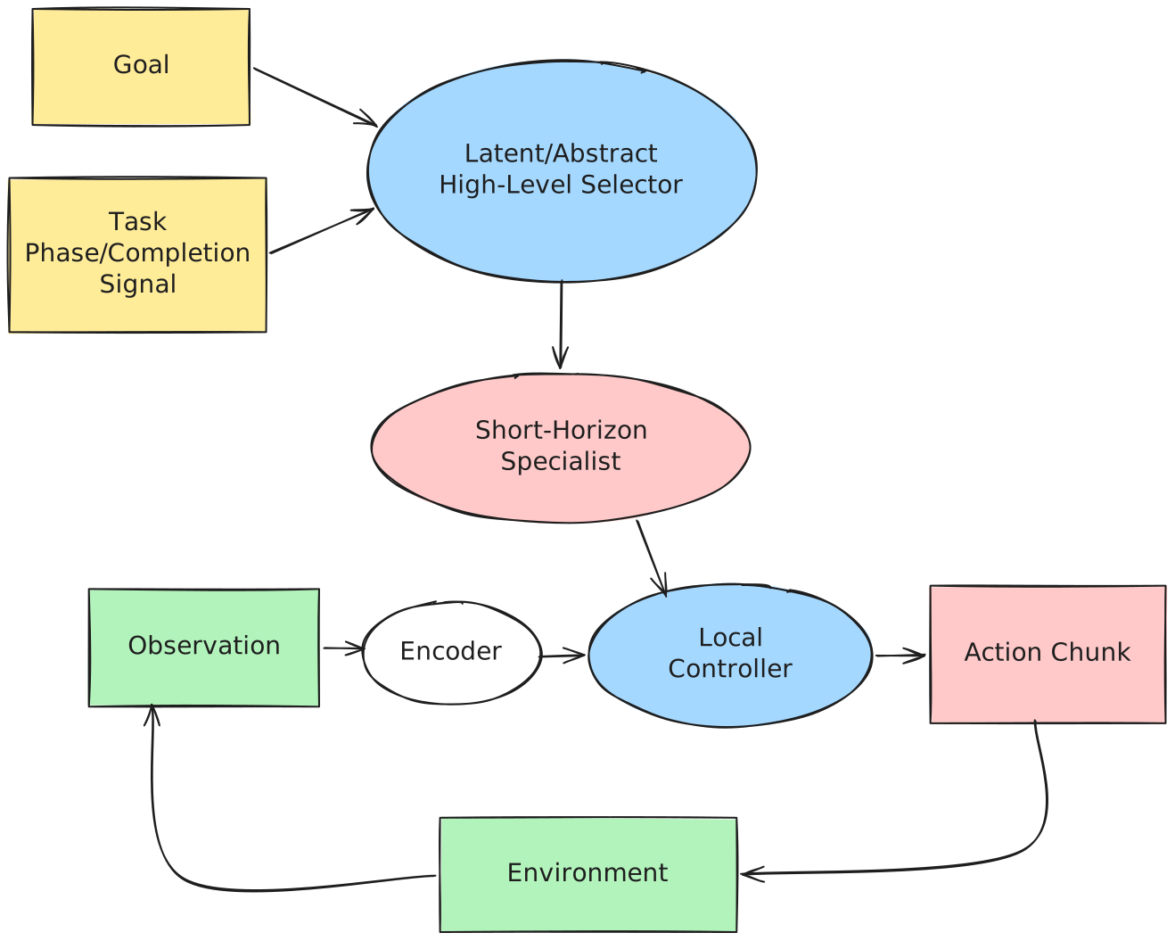
The Slide controller changes the model’s time scale from simulator steps to an impact-to-rest event. Other tasks introduce explicit controller hierarchies for different reasons.
Why direct predictor planning changes across tasks
I first tried to preserve the same-latent coupling of a hierarchical world model: a learned macro-action encoder, a high-level latent predictor, and a future-conditioned inverse low level. This worked for smooth maze-level transitions, where predicted macro futures remain close to demonstrated routes. It did not transfer reliably to contact-rich manipulation.
The issue was not that the predictor had no useful information. In FetchPickAndPlace it could predict a grasp once given an appropriate chunk, but model-predictive control could not discover that precise, temporally extended chunk from a nearly flat pre-contact cost. In FetchSlide, primitive receding-horizon control exploited predictor errors; predicting the single post-strike resting endpoint was more reliable. Similar attempts in Adroit and Kitchen either exploited imagined contact dynamics or merely reproduced an action prior. In these regimes, small prediction errors can become large planning errors when optimization visits off-distribution contact states:
\[\text{small prediction error} \;\not\Rightarrow\; \text{small planning error}.\]The retained controllers therefore keep temporal abstraction but move local control onto future-conditioned action priors, explicit contact modes, or event-level physical predictions. This is not a claim that hierarchical world models cannot solve contact-rich tasks; it is evidence that the compact models, offline data, and planning budgets used here did not support reliable latent model-predictive control there. The corresponding positive and negative runs are documented in Mini-JEPA’s controller discussion and experiment ledger.
Spatial hierarchy
In PointMaze, primitive dynamics are smooth but the route is long. A low-level walker can reach a nearby coordinate; it should not be asked to plan through several walls in one action sequence.
Inspired by Zhang et al.’s hierarchical world model (HWM)
, the maze controller learns a long-timescale latent macro model. Unlike the paper’s fully coupled latent MPC, the retained implementation decodes the predicted macro state into a coordinate subgoal for a learned local walker. A macro-action encoder compresses a primitive chunk,
\[m_t=E_a(a_{t:t+N-1}),\]and a high-level model predicts an abstract latent transition,
\[z^H_{t+N} = z^H_t + g_H(z^H_t,m_t).\]A decoder maps the predicted abstract latent to a local position subgoal. The same proposal lesson reappears at the high level: Gaussian search over macro-actions can invent transitions through walls, so a flow prior samples macro-actions from demonstrated route segments,
\[m_t\sim q_\psi(m\mid z^H_t,p_{\mathrm{goal}}).\]The HWM predicts the next abstract state, the decoder emits a nearby subgoal, and the low-level flow walker reaches it. In checked runs, this fully neural controller reached 1.00 success on PointMaze UMaze, Medium, and Large without storing a reachability graph.
The same route-planning/local-control split is useful in AntMaze, where the walker must reach a sequence of feasible subgoals rather than head directly through walls toward the final goal.
Physical-mode hierarchy
Adroit Relocate needs a different factorization. Reaching for a ball and transporting a held ball are not two points on one smooth action manifold: they are different physical modes.
A single inverse model blurred three regimes: reach, establish possession, and transport/place. The successful controller instead uses two segment-pure future-conditioned inverse specialists:
- a reach specialist, trained only before firm possession and emphasizing live palm-to-ball geometry;
- a held specialist, trained only after firm possession and emphasizing live ball-to-target geometry.
A conservative palm-to-ball threshold of $0.045$ determines firm possession and switches between the specialists. The threshold is deliberately strict: switching early would hand a marginal grasp to the transport specialist, which commonly caused drops. Each specialist tracks one demonstrated future trajectory rather than jumping to whichever demonstration frame is nearest at every replan.
This controller reached 201 successes in 210 held-out episodes (0.957). A single model trained across reaching, acquiring the ball, and transporting it tended to interpolate between incompatible action chunks. Separate specialists give each controller a narrower, more consistent action distribution.
The same future-conditioned inverse-control recipe can be phase-conditioned for Adroit Door, where the controller must distinguish parts of the door-opening sequence.
Door demonstrations are divided into four monotone progress phases corresponding to distinct portions of the opening sequence. At each replan, the controller retrieves a phase-compatible state eight steps in the future and passes the current and target JEPA latents, together with the phase features, to an $H=8$ inverse model.
The predicted action chunk is executed directly before the target is refreshed. This worked because Door follows a stable progression around one articulated object; mixing every phase into one inverse problem produced a less consistent action distribution.
Task hierarchy
FrankaKitchen composes several object interactions. Here the hierarchy is not only temporal or physical; it also decides which task should happen next.
The low level again uses segment-pure inverse specialists, one for each object. A learned completion probe consumes the frozen JEPA latent plus normalized state and decides when to advance. Inside a specialist, a demo-locked future index gives the inverse model a consistent local trajectory to follow.
The harder problem is task order. Greedily selecting the specialist whose demonstrations look closest to the current arm pose ignores the state in which that specialist will finish. Instead, the controller builds a directed handoff graph from demonstration boundaries.
For tasks $a$ and $b$, define the edge cost
\[c(a\rightarrow b) = Q_{0.25} \left( \min_{y\in\operatorname{Start}(b)} \left\| \mathcal N(x)_{0:9}-\mathcal N(y)_{0:9} \right\|_2 \;:\; x\in\operatorname{End}(a) \right).\]The arm-joint slice $0{:}9$ measures handoff reachability. The lower quantile makes the edge robust to outlier demonstrations while asking whether the handoff is well represented somewhere in the data.
A subset dynamic program then solves
\[\pi^\star = \underset{\pi\in\operatorname{Perm}(S)}{\arg\min} \left[ c_{\mathrm{start}}(\pi_1) + \sum_{i=1}^{|S|-1}c(\pi_i\rightarrow\pi_{i+1}) \right]\]for the requested task subset $S$.
When given the deliberately scrambled four-task request
slide, light, microwave, kettle
the demonstration-derived handoff costs select
microwave -> kettle -> light -> slide
With the learned completion probe and live demo re-locking, this controller completed all four tasks in 80 of 100 fresh episodes across four seed blocks. This is a narrower and more defensible claim than “arbitrary task order”: the controller discovers a well-supported order for a requested subset, while the demonstrations still determine which handoffs are feasible.
Results
The table collects the results that directly support the architectural story. Success definitions differ by environment, so rows should be read within a task, not as a leaderboard across tasks.
| Environment | Controller | Checked result | Architectural point |
|---|---|---|---|
| FetchPush | future-conditioned flow + JEPA ranking | 30/30; ~8 mm final distance | propose on the action manifold |
| FetchPickAndPlace | inverse chunk prior + JEPA ranking | 30/30; ~11 mm final distance | prediction is not inverse control |
| FetchSlide | goal-frame event HWM | 0.853 over 2,000 | predict impact-to-rest, not frames |
| PointMaze UMaze / Medium / Large | flow-macro HWM + flow walker | 1.00 / 1.00 / 1.00 in checked runs | separate routing from local control |
| Adroit Door | four-phase future-conditioned inverse | 30/30 | preserve monotone contact progression |
| Adroit Relocate | reach/held inverse specialists | 201/210 | separate physical modes |
| FrankaKitchen, four tasks | handoff graph + inverse specialists + learned completion | 80/100 on scrambled request | compose tasks using demonstration-derived handoffs |
Protocol-aligned external baselines
I also evaluated frozen controllers for 100 fresh episodes and aligned the metric, horizon, task, and reset protocol with published reference results. This is a useful comparison, but not a same-codebase leaderboard: the Gymnasium-Robotics ports contain fixes and are not binary-identical to the older D4RL and Fetch environments used by the literature anchors.

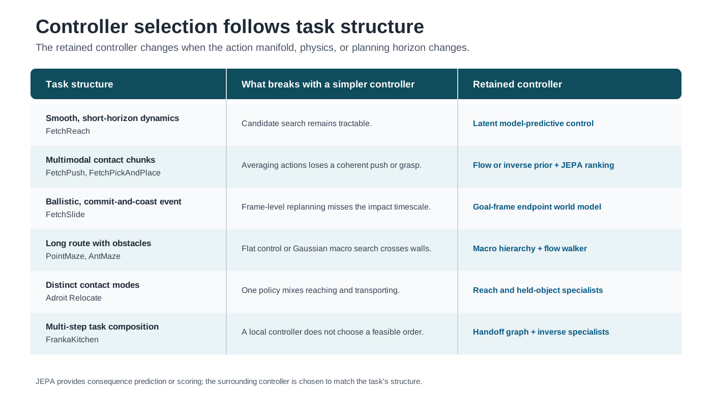
Controller selection map
Conclusion
These experiments suggest that a compact JEPA can play several useful roles in robot control, but that no single planning strategy works across every physical regime.
On smooth, locally controllable dynamics, the learned predictor can directly evaluate action sequences. For FetchPush and FetchPickAndPlace, future-conditioned action priors provide plausible chunks for JEPA to rank. On the more contact-rich Relocate and Kitchen tasks, direct inverse specialists were more reliable than planning through predicted contact dynamics. Ballistic motion benefits from predicting an event endpoint rather than every intermediate frame, while long-horizon navigation and manipulation require explicit temporal, physical-mode, or task-level structure.
The strongest results reflect those distinctions. Flow and inverse proposals with JEPA ranking reached 30/30 on FetchPush and FetchPickAndPlace. The goal-frame FetchSlide model reached 0.853 over 2,000 trials. A learned macro model solved the checked PointMaze layouts, while phase-specific, possession-specific, and task-specific inverse controllers produced the strongest Adroit Door, Adroit Relocate, and Kitchen results.
The protocol-aligned evaluation shows that these compact models can be competitive with selected published baselines, particularly on Fetch and Kitchen, although the environments are aligned rather than binary-identical and the strongest AntMaze and Relocate baselines remain ahead. The broader result is therefore not that one compact JEPA solves robotics generally, but that useful predictive representations can support different controllers when the planning abstraction matches the task’s physics.
Next Steps
These experiments show that compact JEPA representations can support difficult control problems when paired with task-appropriate controllers.
A natural next step is to learn more of the structure that is currently supplied manually. For FetchSlide, model scores could iteratively refine the candidate-strike distribution instead of selecting from a fixed grid. For Adroit and Kitchen, a latent option model could predict the consequences of each specialist and choose contact modes or task handoffs from those predictions. A further test would replace simulator states with visual observations and evaluate whether the same abstractions transfer to harder dexterous tasks such as block and egg manipulation.
Enjoy Reading This Article?
Here are some more articles you might like to read next:
- Reverse Engineering a Star Battle ASIC
- a post with plotly.js
- a post with image galleries
- a post with tabs
- a post with typograms
- a post that can be cited
- a post with pseudo code
- a post with code diff
- a post with advanced image components
- a post with vega lite